When I used to read fairy tales, I fancied that kind of thing never happened, and now here I am in the middle of one!
— Lewis Carroll, Alice in Wonderland
Author: V. Firsanova
Translations: Russian
One of the questions I get asked all the time is what is the best way to start practicing Machine Learning (ML). I wish I had known the answer when I was training my first neural network model! Honestly, I'm a practicing ML researcher and educator, and I still do not have the answer. Right or wrong, I usually suggest newbies trying to train a Convolutional Neural Network (CNN). This elegant architecture helped me get the intuition behind ML. In this post, we'll go through the steps to train a CNN for sentiment analysis using Python. Sentiment analysis is a popular Natural Language Processing (NLP) task that involves classifying text into categories such as positive, negative, or neutral.
How convolutional neural network works
A Convolutional Neural Network (CNN) processes structured grid data such as images. Still, it works great on other types of natural signal data, such as texts. CNNs learn to detect patterns of an object by applying convolutional filters called kernels. We can use these patterns to perform object categorization. For example, we can teach our model to distinguish cats and dogs based on their features (like paws and whiskers). But what is convolution?
Convolution is a mathematical operation that combines two functions (or signals) to produce a third one. For example, image convolution combines an initial image (the first signal) with a kernel (the second signal; think of it as a mask to highlight edges, effects, or other specific features or patterns) to produce a feature map (the third signal) indicating the most significant features such as edges of a depicted object for further processing (or paws and whiskers for image categorization!).
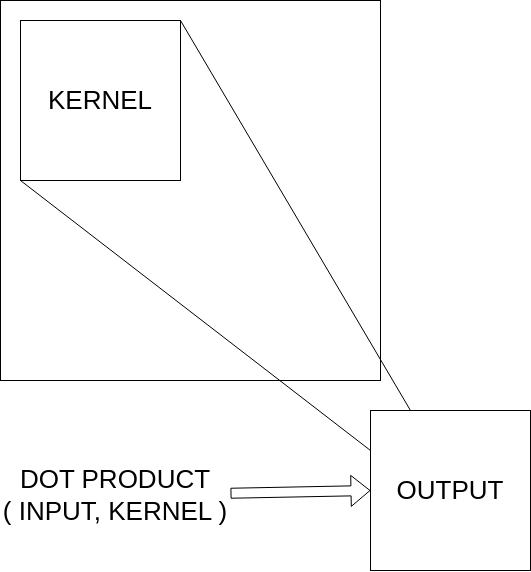
Let's take a detailed look on the convolution operation. As you remember, we need three components (functions or signals):
Kernel: A small matrix (e.g., 3x3, 5x5) designed to extract patterns or features from the input data such as object edges or textures in images. In CNN, kernels contain learnable weights adjusted during the model training to capture the significant features.
Input: Vectorized input signal, for example, 2D array of pixel values representing a grayscale image or a 3D array representing height, width, and RGB channels.
Feature Map: The kernel slides over the input data. At each position, an element-wise multiplication is performed between the kernel and the corresponding input values. The result produces the output feature map.
Essentials on text classification
Text Classification is assigning categories (classes or labels) to a given text. Sentiment analysis, topic labeling, and language detection are common types of text classification in NLP.
Let's look at the main stages of the machine learning procedure:
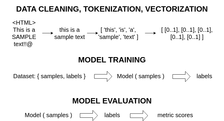
Data Processing:
(1) Data cleaning and text pre-processing for removing artifacts such as HTML tags, filtering unimportant information such as stop-words, converting to lower-case, etc.;
(2) Tokenization, i.e. splitting text into individual tokens (characters, words, subwords, sentences, etc.);
(3) Vectorization, i.e. converting the tokens into numerical vectors for machine processing.
Model Training: Applying machine learning algorithms such as CNN to learn features from the vectorized data and solve the target task, for example, perform sentiment analysis.
Model Evalutation: Getting the outputs using learned model weights to assess the model performance based on evaluation metrics, such as Precision, Recall, and F-Score.
Let's train
Now we'll go through the steps to train a CNN for sentiment analysis using Python and TensorFlow. We're going to use IMDB Reviews Sentiment Analysis dataset. Feel free to download this dataset or use different data.
1. Setting up the device: working on GPU
First, we need to set up GPU:
import tensorflow as tf
# Get a list of all physical devices (e.g., CPU, GPU)
physical_devices = tf.config.list_physical_devices()
# Iterate through each device in the list and print its information
for device in physical_devices:
print(device)Now, by default, training will run on the GPU. Don't forget to enable GPU access in your Colab environment: `Runtime - Change runtime type - T4 GPU`.
2. Dataset: downloading dataset from Kaggle
Next, we need to load and prepare the dataset. For this example, we will use a sample dataset of movie reviews:
# Import the `zipfile` module for working with ZIP archives
import zipfile
# Open the 'IMDB Dataset.csv.zip' ZIP archive in read mode
with zipfile.ZipFile('IMDB Dataset.csv.zip', 'r') as zip_ref:
# Extract all files from the archive into the 'dataset' folder
zip_ref.extractall('dataset')3. Exploratory data analysis: using data analysis methods to define variables for machine learning
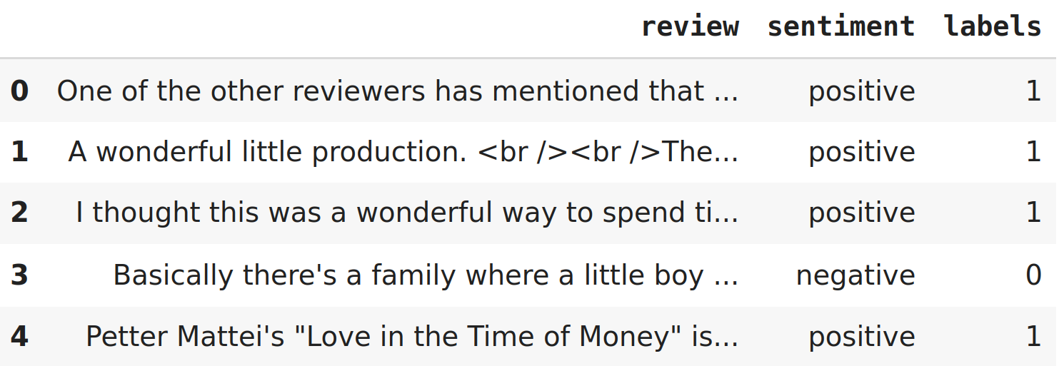
Let's look at our data:
# Import the pandas library for data manipulation
import pandas as pd
# Specify the path to the CSV file
csv_file = '/content/dataset/IMDB Dataset.csv'
# Read data from the CSV file and store it in a DataFrame
data = pd.read_csv(csv_file)
# Display the first 5 rows from the DataFrame
data.head()
Let's examine our data and look at the distribution of text lengths in the dataset.
# Import the matplotlib.pyplot library for data visualization
import matplotlib.pyplot as plt
# Create a new column 'text_len' that contains the text length (number of words) for each review
data['text_len'] = data['review'].apply(lambda x: len(x.split()))
# Create a shape for the graph with size 8x6 inches
plt.figure(figsize=(8, 6))
# Construct a histogram for the distribution of text lengths with 50 bins (the reciprocal of the width of the columns on the graph) and black borders
plt.hist(data['text_len'], bins=50, edgecolor='black')
# Set the label for the X axis
plt.xlabel('Length of Texts')
# Set the label for the Y axis
plt.ylabel('Frequency')
# Set the title for the histogram
plt.title('Histogram of Length of Texts')
# Turn on the grid on the chart
plt.grid(True)
# Show the graph
plt.show()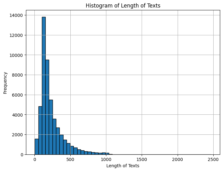
Based on the graph, you can set the upper value of the length of texts in the dataset before processing. Now let's look at the distribution of labels: is the dataset balanced?
plt.figure(figsize=(10, 6))
# Build a bar chart for label distribution
data['labels'].value_counts().plot(kind='bar')
plt.xlabel('Labels')
plt.ylabel('Frequency')
plt.title('Distribution of Labels')
# Rotate the labels on the X axis by 45 degrees for better readability
plt.xticks(rotation=45)
# Turn on the Y axis grid
plt.grid(axis='y')
plt.show()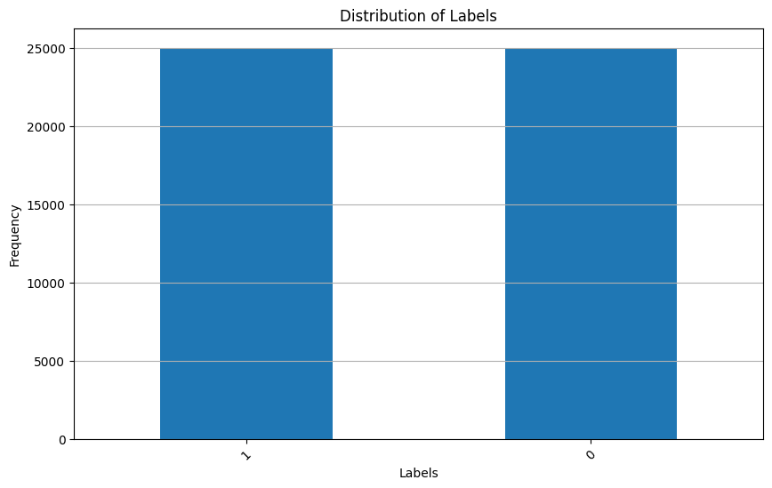
4. Data tokenization and vectorization
Let's write texts and labels into separate variables:
# Extract the column with review texts into the 'texts' variable
texts = data['review']
# Extract the column with labels into the 'labels' variable
labels = data['labels']
# Display the second review and its label (index 1, since indexing starts at 0)
texts[1], labels[1]Let's automate tokenization and vectorization processes using Keras. To perform word-level tokenization we'll set the maximum text length value using the length distribution histogram that we built earlier. We'll use this value to trim all texts exceeding this value to a given length and fill all short texts with zeros to the required length.
Why zeros? This operation called padding is necessary to make all matrices representing texts of the same length. Machine learning is based on matrix operations, and all the matrices must be the same size in order to be multiplied.
# Import the necessary classes from the TensorFlow Keras library for working with text data
from tensorflow.keras.preprocessing.text import Tokenizer
from tensorflow.keras.preprocessing.sequence import pad_sequences
# Create a Tokenizer object
tokenizer = Tokenizer()
# We train the tokenizer using review texts
tokenizer.fit_on_texts(texts)
# Convert review texts into sequences of numbers (word indices)
X = tokenizer.texts_to_sequences(texts)
# Set the maximum length of sequences
max_len = 500
# Append or trim sequences to a given maximum length
X = pad_sequences(X, maxlen=max_len)
# Convert the labels to a numpy array
y = labels.values
X[1], y[1]Now, let's create three samples using sklearn: training, validation and test sets.
# Import the train_test_split function from the sklearn library
from sklearn.model_selection import train_test_split
# Split the data into a training sample (60%) and a temporary sample (40%)
X_train, X_temp, y_train, y_temp = train_test_split(X, y, test_size=0.4, random_state=42)
# Split the temporary sample into validation (20%) and test (20%) samples
X_val, X_test, y_val, y_test = train_test_split(X_temp, y_temp, test_size=0.5, random_state=42)
# Output the sizes of training, validation and test samples
print(f"X_train shape: {X_train.shape}, y_train shape: {y_train.shape}")
print(f"X_val shape: {X_val.shape}, y_val shape: {y_val.shape}")
print(f"X_test shape: {X_test.shape}, y_test shape: {y_test.shape}")Let's look at the tokenization result: what does the training dictionary look like?
# Output tokenizer dictionary elements representing word indexing
# from 51 to 55 (indexing starts from 0)
list(tokenizer.word_index.items())[50:55]Set machine learning parameters: the size of the dictionary will be equal to the size of the embedding (vector representation).
# Calculate the size of the dictionary;
# add 1 due to indexing from 1 (usually it starts from 0)
vocab_size = len(tokenizer.word_index) + 1
vocab_sizeThe next parameter is the number of classes, or categories
# Calculate the number of unique classes in labels y
num_classes = len(set(y))
num_classesSet the dimension of the embedding matrix: the larger this value, the deeper our machine learning model is, the more features it can detect in the data. But the larger this value, the longer the model will take to train.
embedding_dim = 100Maximum sequence length: we have already set this parameter earlier.
max_len5. Model training
Let's set out model:
# Import the necessary classes from the TensorFlow Keras library
from tensorflow.keras.models import Sequential
from tensorflow.keras.layers import Embedding, Conv1D, GlobalMaxPooling1D, Dense
# Create a sequential model
model = Sequential([
# Embedding layer for creating word embeddings
Embedding(vocab_size, embedding_dim, input_length=max_len),
# Conv1D layer for convolution on one-dimensional sequences
Conv1D(128, 5, activation='relu'),
# GlobalMaxPooling1D layer to extract features from the convolutional layer
GlobalMaxPooling1D(),
# Fully connected layer with 10 neurons and ReLU activation function
Dense(10, activation='relu'),
# Output fully connected layer with num_classes neurons and softmax activation function
Dense(num_classes, activation='softmax')
])
# Compile the model with the Adam optimizer,
# the sparse_categorical_crossentropy loss function and the accuracy metric
model.compile(optimizer='adam',
loss='sparse_categorical_crossentropy',
metrics=['accuracy'])
# Output the structure of the model
model.summary()This is our model summary:
| Layer (type) | Output Shape | Param # |
|---|---|---|
| embedding (Embedding) | (None, 500, 100) | 12425300 |
| conv1d (Conv1D) | (None, 496, 128) | 64128 |
| global_max_pooling1d (GlobalMaxPooling1D) | (None, 128) | 0 |
| dense (Dense) | (None, 10) | 1290 |
| dense_1 (Dense) | (None, 2) | 22 |
Now let's draw the structure of the model.
# Import the plot_model function from the TensorFlow Keras library
from tensorflow.keras.utils import plot_model
# Visualize the structure of the model
plot_model(model)
# Note: To save the model image to the file 'model_plot.png'
# specify show_shapes=True and show_layer_names=True to display layer shapes and their names
# plot_model(model, to_file='model_plot.png', show_shapes=True, show_layer_names=True)
# This code will create an image of your model structure and save it to a file called model_plot.png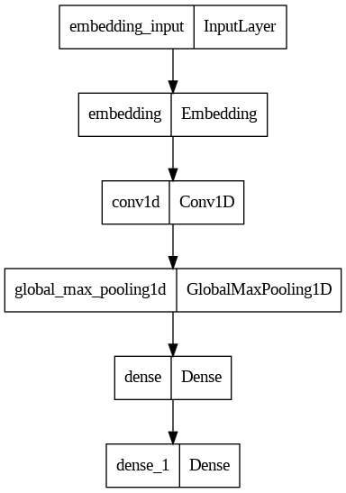
Yay! Let's start training!
This code starts the model training process on the X_train training data with the corresponding y_train labels. During the model training process, one epoch will be performed (epochs=1), the data will be processed in batches of 32 samples (batch_size=32), and validation data will be used from X_val and y_val to evaluate the model performance.
# Train the model using X_train training data and y_train labels
history = model.fit(X_train, y_train, # model training data
epochs=1, # number of training epochs
batch_size=32, # data batch size
validation_data=(X_val, y_val)) # model validation dataLet's evaluate the accuracy of the trained model.
This code evaluates the performance of the trained model on the test dataset (X_test and y_test). The evaluation results include the value of the loss function (loss) and accuracy (accuracy).
# We evaluate the performance of the model on test data X_test and labels y_test
loss, accuracy = model.evaluate(X_test, y_test)
# Display the accuracy on the test sample
f'Test accuracy: {accuracy}'Now, let's get predictions from the test sample.
After this operation is completed, the predictions variable will contain the predicted probabilities for each class for each example in the test dataset.
# Get model predictions on test data X_test
predictions = model.predict(X_test)
predictionsAll these numbers are not human readable at all!
Firstly, the texts are encoded...
def detokenize(tokenized_text, tokenizer):
"""
A function to convert tokenized text back to its original form.
Arguments:
tokenized_text -- tokenized text (list of indices or tokens)
tokenizer -- a tokenizer object containing the index_word dictionary
Returns:
Source text as a string.
"""
index_word = tokenizer.index_word # Get the index_word dictionary from tokenizer
return " ".join(index_word.get(token, '') for token in tokenized_text)Secondly, the predictions are encoded...
import numpy as np
# Use the detokenize function
# to restore the original text from the tokenized sequence X_test[7]
# Use np.argmax
# to determine the class index with the highest probability in predictions[7]
detokenize(X_test[7], tokenizer), np.argmax(predictions[7])6. Confustion matrix
The confusion matrix shows which classes were correctly and incorrectly predicted by the model on the test dataset y_test and predictions.
import seaborn as sns
from sklearn.metrics import confusion_matrix
from sklearn.metrics import ConfusionMatrixDisplay
# Get true labels and predicted labels
true_labels = y_test
predicted_labels = [np.argmax(predictions[i]) for i in range(len(predictions))]
# Define unique class labels
labels = np.unique(true_labels)
# Calculate the confusion matrix
cm = confusion_matrix(true_labels, predicted_labels, labels=labels)
plt.figure(figsize=(8, 6))
# Build a heat map of the error matrix
sns.set(font_scale=1.2) # Set the font scale for better readability
sns.heatmap(cm, annot=True, fmt='d', cmap='Blues', cbar=False,
xticklabels=labels, yticklabels=labels) # Display a matrix with numeric labels
plt.xlabel('Predicted Labels')
plt.ylabel('True Labels')
plt.title('Confusion Matrix')
plt.show()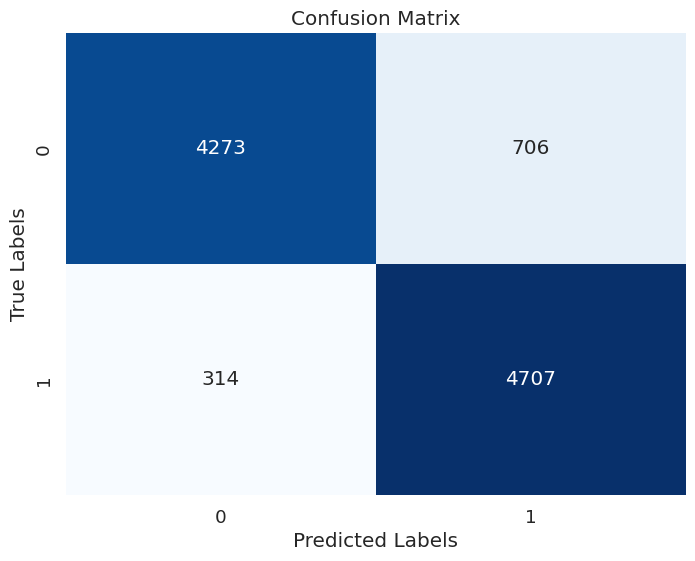
Wow! The results are amazing. Feel free to use and change the code and use different data. Have fun coding!